Lowering Slot Time and Validators Economic

Why This Matters, by Stakeholder

Validators and client teams: shorter slots provide more frequent leader opportunities and lower block-reward variance, but double vote frequency at 200 ms and leave less wall-clock margin for voting and leader handoff
Traders and searchers: shorter slots reduce stale-price arbitrage against external reference markets; the effect on sandwich profitability is ambiguous and depends on reaction latency, market contention, and user slippage
Liquidity providers and market makers: faster state updates reduce stale-price exposure and LVR, while finer slot granularity improves the timeliness of oracle- and quote-driven strategies
Stakers and delegators: validator revenues become more predictable, but higher voting costs and potential TVC sensitivity can redistribute economics across validators with different stake and latency profiles
Protocol and infrastructure teams: current vote timing and leader-handoff tails consume a material fraction of a 200 ms slot, making staged mainnet monitoring essential

TL;DR

Reducing slot time from 400 to 200 ms halves the four-slot leader window from 1.6 s to 800 ms, limiting how long a single execution regime can persist
Shorter slots reduce modeled stale-price arbitrage against external reference markets, with the effect increasing for wider fee bands and lower short-horizon volatility.
- Current snapshot of arbitrage indicates intensive on-chain routing; arbitrage will likely remain unchanged after slot time reduction
Sandwich MEV is not sign-definite: shorter reaction windows reduce attack feasibility, while lower intra-slot contention can leave more residual slippage available to fast attackers
More frequent leader opportunities reduce validator block-reward variance, with a larger reduction in downside uncertainty than in the long-tail upside
At 200 ms, validators vote roughly twice as often per unit of wall-clock time; expected vote-fee recapture thresholds remain similar, but smaller validators face larger absolute voting costs
Current vote timing and leader-handoff distributions leave limited latency headroom at 200 ms, so the impact on TVCs and consensus performance remains an empirical mainnet question

Relevant Charts

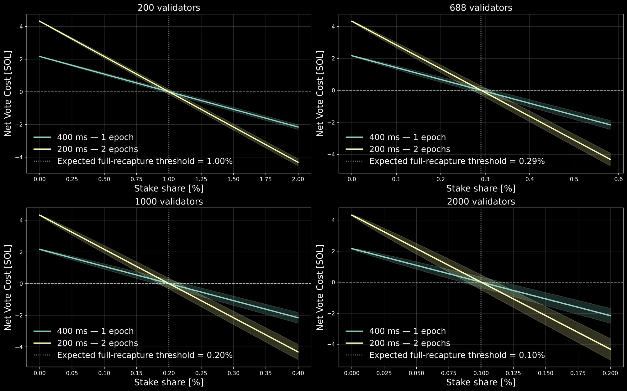
**Net vote-fee cost as a function of stake share and validator-set size.** Simulated net vote cost in SOL, defined as the validator's own vote-fee expenditure minus vote fees redistributed to it during its leader windows. Panels correspond to validator sets of 200, 688, 1,000, and 2,000 validators, assuming one vote transaction per validator per slot. Solid lines show the median outcome; shaded regions span the 5th to 95th percentiles generated by random leader assignment.

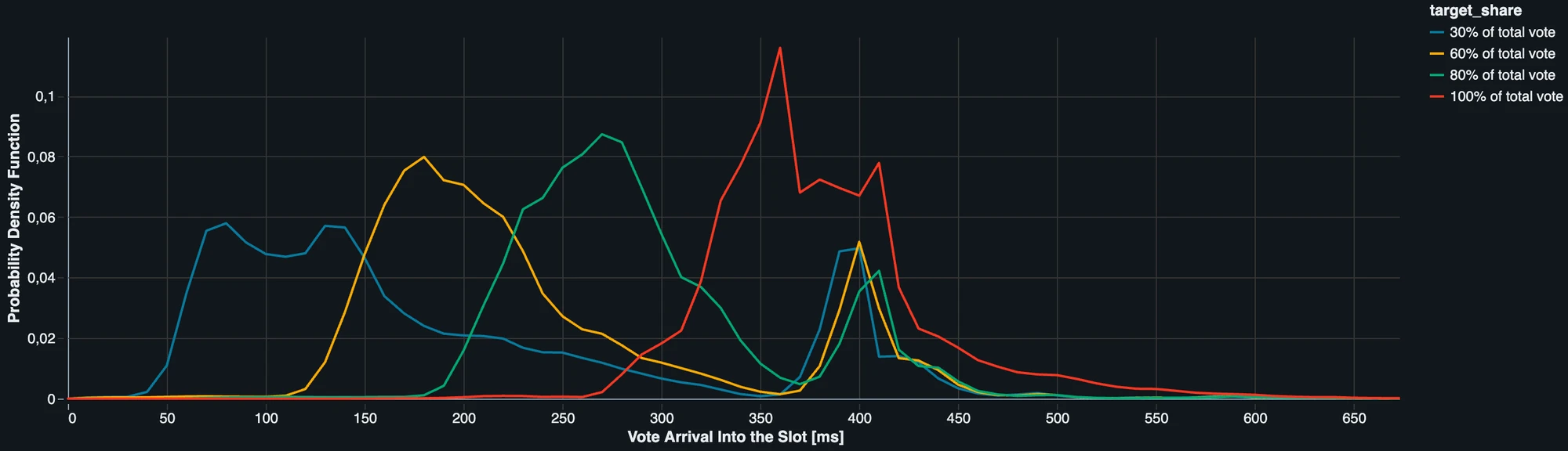
**Within-slot accumulation of vote transactions.** Distribution of the time at which cumulative vote-transaction count reaches 30%, 60%, 80%, and 100% of each eligible slot's observed vote transactions. The unit of observation is a produced slot. Vote arrival time is measured within the slot and threshold times are grouped into 10 ms bins; the y-axis is the share of eligible slots falling in each bin, with each threshold normalized separately.

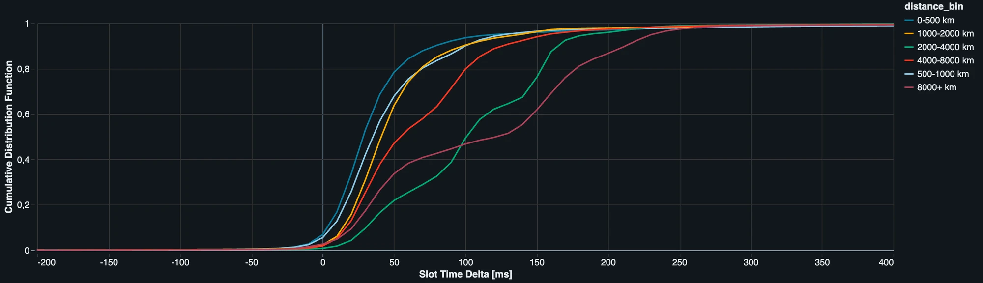
**Additional duration of the first slot after a leader handoff, grouped by geographic distance.** CDF of $(\Delta t=t_0-(t_1+t_2+t_3)/3)$ for four-slot leader windows observed from July 10, 2026 onward. The unit of observation is a valid leader-transition sequence: slot 0 is the first slot produced by a new leader, while slots 1-3 are produced by that same leader. Previous and current leaders are grouped by Haversine distance between reported coordinates. The x-axis is the resulting slot-0 handoff penalty in milliseconds and the y-axis is the cumulative fraction of sequences at or below that penalty. Right-shifted curves indicate slower handoffs.

Introduction

Solana’s performance roadmap is moving around a simple engineering objective: Increase Bandwidth, Reduce Latency (IBRL). Reducing slot time is one of the key feature to tackle the latency-sensitive component of IBRL.

SIMD-0525 proposes reducing the target slot time from 400 ms to 200 ms in four feature-gated stages: 350, 300, 250, and 200 ms. The main economic effect is that blockspace is exposed to the market in smaller and more frequent increments. Information can be incorporated into canonical state more frequently; a single leader controls ordering for less wall-clock time; applications that reason about freshness in slots obtain a finer temporal signal (for example, oracle consumer and propAMM-style market makers).

Another aspect of reducing slot time is to bring consensus latency and inclusion latency much closer once Alpenglow is live. Solana currently targets roughly 400 ms slots, whereas Alpenglow is designed to bring consensus finality toward roughly 150ms (under current stake distribution).

Bringing these two timescale closer together may also remove an otherwise available source of timing optionality. If consensus of block $n$ can be obtained substantially faster than the duration of slot $n+1$ , a sufficiently conservative next leader can, in principle, spend part of its block production interval waiting for a stronger consensus signal before committing to block $n+1$ . With 200 ms slot target, the same wait would consume most of the available interval.

The case for shorter slots is broader than faster confirmations: the temporal structure of execution market is changed. This has potential beneficial consequences for transaction inclusion, stale-price, and liquidity provision. However, it also changes validator economics. The relevant question is consequently not whether reducing slot time is “good” or “bad”, but which parts if the system benefit from finer temporal granularity.

Reducing slot time has been discussed in:

Effects on Market Structure Primitives

The most direct market-structure consequence of SIMD-0525 comes from keeping the leader window fixed at four slots. Reducing slot target from 400 to 200 ms therefore reduces continuous control by a single leader from 1.6 seconds to 800 ms.

Why should this matter?

A block producer controls when transactions are executed and how they are ordered within its blocks. Previous analysis show how some validators are statistically consistent with delayed-execution models for certain type of transactions. This behaviour extends to a variety of Agave and Firedancer/Frankendancer forks. Fig. 1 shows how non-vote transactions are distributed over the slot for different clients. In other words, it shows when a transaction is more likely to be included during the slot. We can see that this timing differs across clients: some are more likely to include transactions near the beginning of the slot, while others concentrate more transactions toward the end.

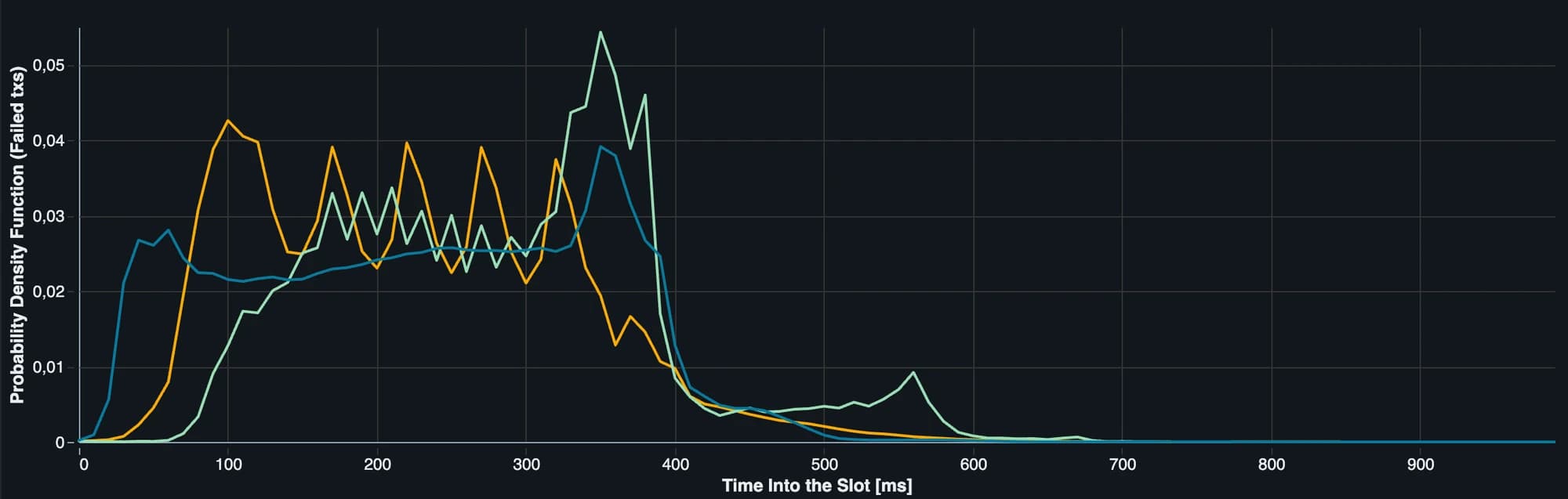
**Fig. 1: Within-slot timing of non-vote transaction inclusion by validator client.** Distribution of non-vote transactions over elapsed time within the slot, separated by validator client implementation. The x-axis reports time into the slot and the y-axis reports the normalized transaction distribution. Differences across curves show that transaction inclusion is not uniform through the slot and that client implementations exhibit distinct timing profiles, particularly near slot boundaries.

From a market-microstructure perspective, delaying execution keeps the on-chain state stale for longer. During that interval, prices can move on external venues, new orders can arrive, and previously submitted quotes can become less representative of current market conditions, cfr. The Scheduler War (Part 1): A Closer View of Solana Microstructure.

Shortening the leader window places a mechanical upper bound on how long any one leader can maintain such an execution regime before another leader gets an opportunity to produce blocks.

Persistent slow-execution regimes

To isolate this mechanism, we consider a deliberately stylized model. Suppose that a fraction $p_\text{slow}=0.33$ of leader windows use a scheduler that systematically delays transaction execution, and suppose for the moment that scheduler type is independently assigned across leader window.

Let $M$ denote the maximum number of consecutive slow-scheduler leader windows observed over a fixed wall-clock horizon. We compare two approximately 48-hour periods:

400 ms slots: 432,000 slots corresponding to 108,000 four slot leader windows of 1.6 seconds each
200 ms slots: 864,000 slots across two shorter epochs, corresponding to 216,000 four-slot leader windows of 800 ms each.

Holding wall-clock time fixed is important here. At 200 ms, SIMD-0525 keeps 432,000 slots per epoch, so a single epoch last only about one day.

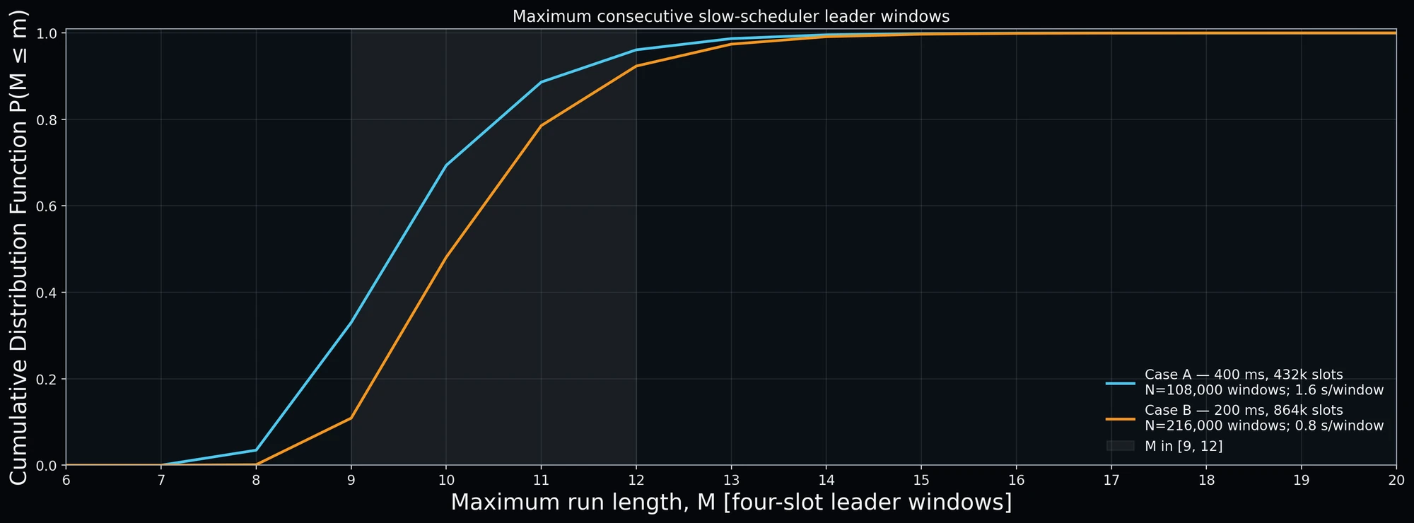
**Fig. 2:** **Maximum run length of consecutive slow-scheduler leader windows.** Cumulative Distribution Function (CDF) of the maximum number of consecutive slow-scheduler leader windows over an approximately 48-hour horizon, under an independent Bernoulli model with $p_\text{slow}=0.33$ . The 400 ms case contains 108,000 four-slot leader windows; the 200 ms case contains 216,000 windows across two shorter epochs. For any x-axis value m, the CDF gives the probability that the longest slow-scheduler run contains at most m consecutive leader windows.

Figure 2 shows the CDF of maximum number of consecutive slow-scheduler leader windows. Because the 200 ms configuration contains twice as many leader windows over the same 48-hour horizon, its maximum run is not mechanically smaller when expressed as a number of windows. In fact, more draws create somewhat more opportunity to observe a longer run. Under the model, the maximum run lies between 9 and 12 windows with approximately 92.6% probability in the 400 ms case and approximately 92.2% in the 200 ms case.

This is not, however, the economically relevant unit.

A slow window lasts 1.6 seconds under current configuration and 800 ms under the proposed endpoint. Figure 2 therefore maps exactly the same run-length experiment into wall-clock duration. A sequence of 9-12 slow leader windows corresponds to 14.4-19.2 seconds at 400ms slots, but only 7.2-9.6 seconds at 200 ms slots. The distribution shift sharply once the x-axis is expressed in seconds rather than leader windows.

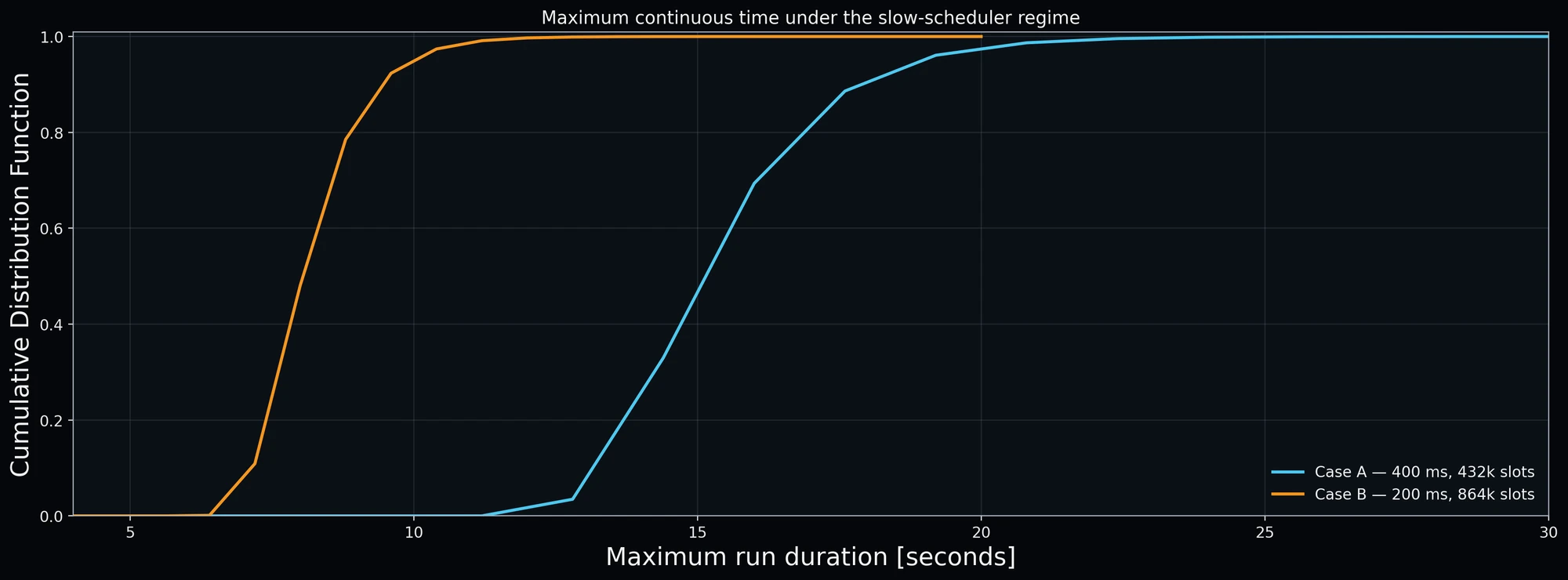
**Fig. 3:** **Maximum continuous duration of slow-scheduler regimes.** CDF of the same maximum-run model shown in Fig. 2, converted from leader-window counts into wall-clock duration. Each leader window lasts 1.6 s at 400 ms slots and 0.8 s at 200 ms slots. The x-axis reports the maximum continuous duration of a slow-scheduler sequence in seconds; the y-axis gives the probability that the longest such sequence is no longer than that duration.

This is the mechanism that matters for market structure. Shorter slots do not necessarily prevent a sequence of leaders using the same execution policy. They reduce the amount of continuous wall-clock time represented by that sequence.

Thus, for a fixed sequence of leader-level execution regimes, halving the duration of each leader window mechanically compresses the time over which an unfavorable regime can persists.

This is already economically relevant. In electronic markets, information decay is measured in time, not in blocks. A ten-window stale execution regime is substantially less damaging if it lasts 8s rather than 16s.

Faster blocks reduce stale-price arbitrage

The same time compression applies to a second mechanism: cross-venue arbitrage. Here the venue is dependent from an off-chain clock (another blockchain or a CEX).

Consider an AMM whose on-chain price is aligned with an external reference price, immediately after block. Between blocks, the reference price continues to evolve while the AMM state remains unchanged. An arbitrage opportunity appears once the external price has moved sufficiently far to overcome the AMM’s trading fee. Longer block intervals therefore give the external price more time to leave the no-arbitrage region before the next opportunity to update the pool.

Milionis et al formalized this mechanism for AMMs with fees and discrete Poisson block arrivals. The resulting closed form for profits is a function of the volatility of the underlying asset, the block arrival rate, and fee.

Figure 4 shows how the arbitrage profits as a function of fee, volatility, and block time. The four panels correspond to trading fee of 1, 5, 10, and 30 basis points, while each panel contains curves for daily volatility of 1%, 5%, 10%, and 20%. Every curve reports the reduction in modeled constant-product AMM arbitrage intensity relative to the 400 ms baseline as the target slot time moves through the SIMD-0525 stages.

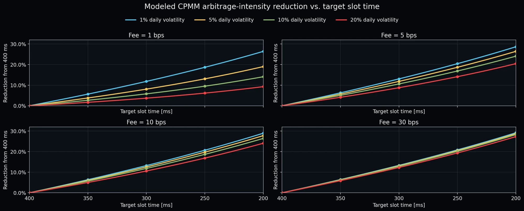
**Fig. 4:** **Modeled reduction in constant-product AMM stale-price arbitrage under shorter slots.** Reduction in normalized arbitrage-profit intensity relative to a 400 ms baseline, evaluated using the discrete-block AMM model of Milionis et al. The x-axis is target slot duration. Panels correspond to trading fees of 1, 5, 10, and 30 bps, while curves within each panel correspond to daily volatility of 1%, 5%, 10%, and 20%. Positive values indicate lower modeled arbitrage extraction as slot time decreases. The result applies to an on-chain AMM arbitraged against an external reference price evolving between blocks.

When the no-arbitrage band is wide relative to short-horizon price volatility, price needs more time to diffuse far enough to make an arbitrage profitable, and reducing the available interval has a comparatively large effect. With very low fees or high volatility, profitable deviations emerge more easily, so shortening the block interval removes a smaller fraction of opportunities.

It is worth mentioning that, the current environment of arbitrages on Solana is richer than this simple case. In the last 5 days, ~36% of the arbitrage profits were realized using pure on-chain venues, although more than 60% of total volume routed via propAMM (see Fig. 5). This clearly indicate that arbitrage snapshot can very likely remain the same post slot time reduction.

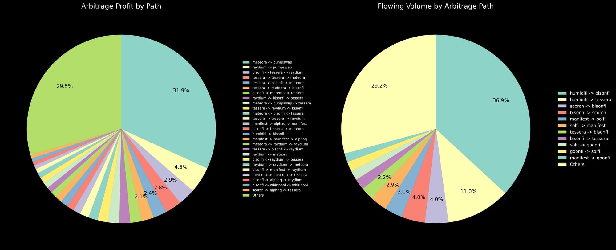
**Fig. 5:** **Composition of observed atomic arbitrage profit and flowing volume by route.** Share of total observed atomic-arbitrage profit (left) and flowing volume (right) attributed to each arbitrage path in the Dune sample. Routes are ranked separately for each metric; paths are shown individually until cumulative contribution exceeds 70%, with the remaining routes aggregated into Others. Percentages therefore represent shares of total profit or total flowing volume, respectively, and the path composition need not be the same across the two panels. The figure shows that profit concentration and routed-volume concentration are distinct. Source: Dune.

Implication on Sandwiching

The effect of shorter slots on sandwich MEV is less straightforward than the effect on stale-price arbitrage.

A simple timing argument would suggest that reducing slot duration makes sandwiching harder. If an attacker needs $d$ milliseconds to observe a victim transaction, construct the attack, and submit it, then shortening the interval available before the end of the slot reduces the fraction of transactions for which the attacker can react in time.

This captures only one part of the mechanism.

A transaction waiting inside a slot is also exposed to other transactions affecting the same market. Those transactions may consume part of the victim's slippage tolerance before the victim is executed. A shorter slot reduces this market-local contention. If users keep the same slippage tolerance, the victim may therefore reach execution with more residual slippage available, increasing the amount that a sufficiently fast attacker can extract.

Appendix A develops a closed-form model combining these two channels. Slot duration enters through

\mu=\lambda\tau,

where $\lambda$ is the rate of transactions relevant to the same market and $\tau$ is slot duration, and through

\rho=\frac{d}{\tau},

which measures attacker reaction latency relative to the available slot time.

Reducing $\tau$ lowers $\mu$ , reducing pre-victim contention, but increases $\rho$ , reducing the time available to react. The two effects work in opposite directions.

A third channel appears if users adapt their slippage settings to expected contention. We parameterize this response through $\kappa$ : larger values mean that the victim exposes less slippage as expected intra-slot contention falls.

Figure 6 explores these interactions jointly rather than varying one parameter at a time. Each Monte Carlo draw combines an attacker reaction latency $d$ , a market-local arrival rate $\lambda$ , a slippage-adjustment parameter $\kappa$ , a baseline slippage-to-impact ratio $D_0$ , and a normalized attack cost $\phi$ . For each draw, the model is evaluated at both 400 ms and 200 ms.

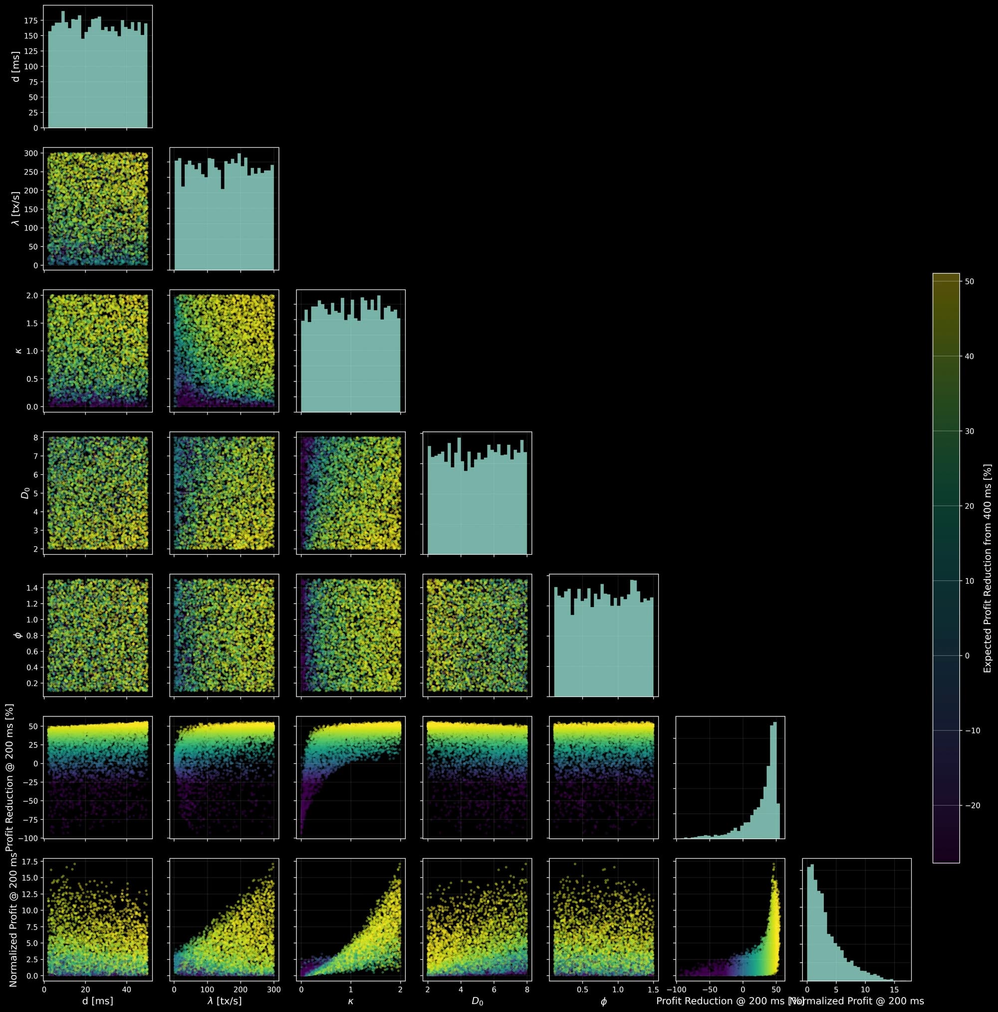
**Fig. 6:** **Joint sensitivity of modeled sandwich profitability to shorter slots.** Lower-triangle Monte Carlo sensitivity plot for the slot-level sandwich model in Appendix A. Each point represents one joint draw of attacker reaction latency ( $d$ ), market-local relevant transaction rate ( $\lambda$ ), slippage-response parameter ( $\kappa$ ), baseline slippage-to-impact ratio ( $D_0$ ), and normalized fixed attack cost ( $\phi$ ). Diagonal panels show the sampling distribution assigned to each parameter or output; off-diagonal panels show pairwise relationships. Point color reports the modeled change in expected sandwich profit when moving from 400 ms to 200 ms

The result is not sign-definite. Some combinations produce lower expected sandwich profit at 200 ms; others produce higher profit. The clearest separation occurs along the slippage-response dimension. When slippage remains relatively insensitive to lower contention, reducing the number of transactions preceding the victim can leave more extractable headroom and offset the shorter reaction window. As slippage adapts more strongly, this effect reverses: the victim exposes less headroom while the attacker simultaneously has less time to react.

Reaction latency provides the second important separation. For very low-latency attackers, moving from 400 to 200 ms removes only a small fraction of their feasible reaction window. For slower attack paths, the same slot-time reduction consumes a materially larger fraction of the available interval.

The model therefore gives a different conclusion from stale-price arbitrage. Shorter slots mechanically reduce the time over which an AMM can remain stale relative to an external price, but they do not mechanically reduce sandwich profitability. The latter depends on how execution contention, user slippage, attacker latency, and ordering behavior interact.

The Monte Carlo should not be interpreted as estimating the probability that sandwich MEV will rise or fall. The parameter draws are sensitivity ranges rather than empirically calibrated distributions. Empirically determining the sign therefore requires transaction-level calibration of slippage, market-local activity, price impact, attacker latency, and bundle-ordering success.

Validator economics

Shorter slots also change the economics of operating a validator. Two mechanisms move in different directions.

First, more frequent leader opportunities reduce the randomness associated with block production. Second, until on-chain voting is removed from the critical path, faster slots require validators to vote more frequently per unit of wall-clock time.

The first effect improves revenue predictability. The second increases operating expenditure and changes the distribution of vote-fee transfers across validators

A validator receives leader opportunities approximately in proportion to stake, but realized block rewards are noisy. Even over an epoch, a small validator may receive more or fewer leader windows than expected, and those windows do not all carry the same economic value.

Figure 7 isolates this sampling effect for a validator with a 0.1% stake share. It simulates leader rewards using four-slot leader windows and a fixed observed reward pool. The 400 ms case uses the current leader cadence; the 200 ms proxy exposes the validator to more, shorter leader windows over the corresponding wall-clock horizon.

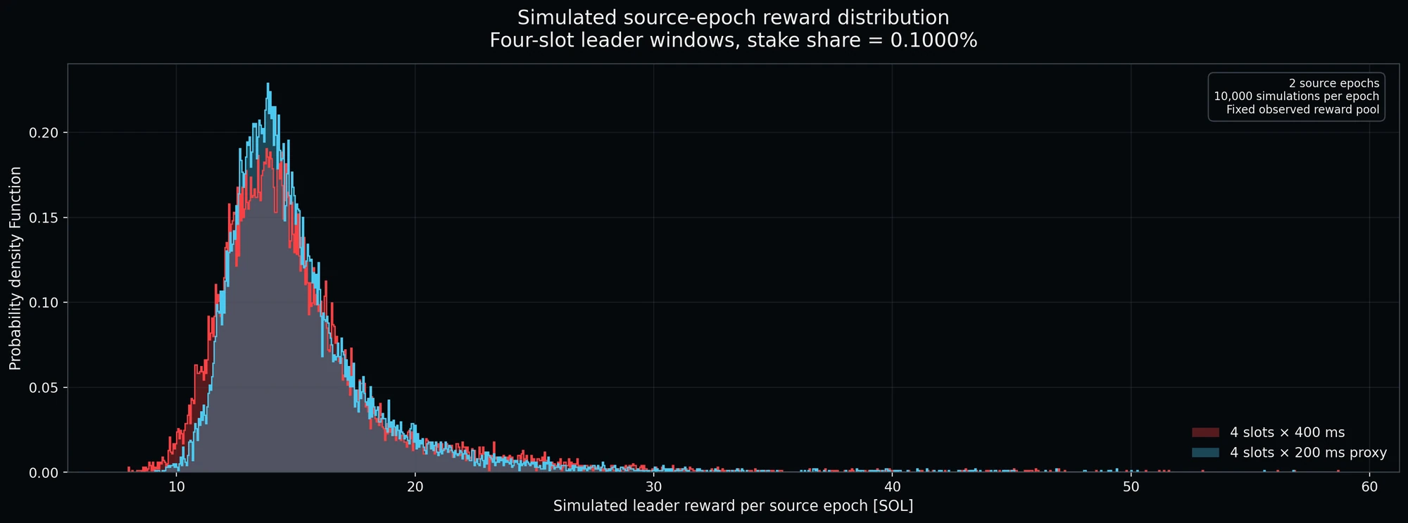
**Fig. 7:** **Simulated distribution of leader rewards under 400 ms and 200 ms slot cadences.** Distribution of simulated block-production revenue for a validator with 0.1% stake, using four-slot leader windows and a fixed observed reward pool. The unit of observation is one simulated source epoch; the figure uses 10,000 simulations per source epoch over two source epochs. The 400 ms curve represents the current four-slot leader cadence, while the 200 ms curve is a shorter-slot proxy with more leader opportunities over the corresponding wall-clock interval. The y-axis is probability density and the x-axis is simulated leader reward in SOL. The tighter 200 ms distribution shows lower sampling variance. Because the underlying reward distribution has a long right tail, variance compression is asymmetric: downside dispersion contracts more strongly than the rare high-reward upside.

The central effect is a reduction in dispersion. With more independent leader opportunities, realized reward converges more tightly toward its expectation. In practical terms, shorter slots make block-production revenue more predictable for a fixed stake share.

The improvement is not symmetric around the center of the distribution. Observed block rewards are long-tailed: most leader windows generate rewards close to the center of the distribution, while a smaller number produce unusually large rewards. Increasing the number of leader opportunities therefore removes more of the downside generated by receiving too few or unusually weak windows than it removes of the upside generated by landing one of the rare high-reward windows.

Consequently, the contraction in the lower tail is larger than the contraction in the upper tail. Shorter slots reduce reward variance, but the long-right-tail structure of block rewards means that this reduction is asymmetric.

This is a distributional effect rather than a claim that shorter slots mechanically increase expected block revenue. The simulation holds the reward pool fixed; it measures how frequently a validator samples that pool, not how the underlying fee market responds to a different slot cadence.

The same increase in temporal granularity has a direct cost for validators: at 200 ms, a validator that votes once per slot submits approximately twice as many vote transactions per unit of wall-clock time as at 400 ms.

Part of those fees is burned and part is redistributed to leaders. A validator can therefore recover some or all of its own vote-fee expenditure when it receives leader windows and collects the vote fees paid by the rest of the validator set.

Figure 8 shows, for a given stake share, what is the probability that a validator receives enough leader windows to fully recapture its own vote-fee expenditure from redistributed vote fees.

Under the assumptions of the model, comparing one 400 ms epoch with two 200 ms epochs over approximately the same wall-clock horizon does not materially move the expected full-recapture threshold. Vote expenditure doubles, but so does the number of leader opportunities through which vote fees can be recovered.

What changes is the variance around that threshold.

At 200 ms, the CDF becomes steeper. For stake shares below the expected full-recapture point, the probability of getting sufficiently lucky leader assignments decreases. For stake shares above it, the probability of fully recapturing vote fees increases. The shorter cadence therefore removes part of the leader-schedule lottery around the expected value.

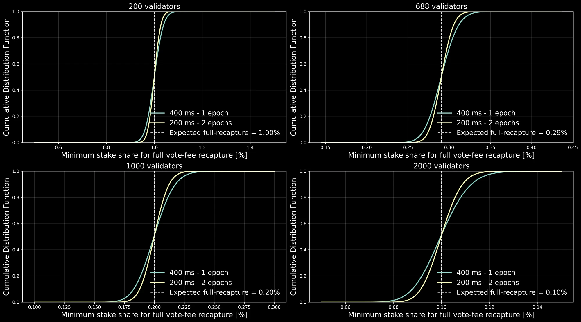
**Fig. 8:** **Probability of fully recapturing vote-fee expenditure through leader assignments.** CDF of the minimum stake share required for redistributed vote-fee revenue to cover a validator's own vote-fee expenditure. Each panel assumes a different validator-set size - 200, 688, 1,000, or 2,000 validators - with one vote transaction per validator per slot. The 400 ms case covers one 432,000-slot epoch; the 200 ms case covers two 432,000-slot epochs, keeping the nominal wall-clock comparison approximately fixed. At any x-axis value, the CDF gives the probability that the realized leader schedule is sufficient for full vote-fee recapture at that stake share. The vertical line marks the expected recapture threshold.

Full recapture is only one point on the distribution. Figure 9 therefore shows the more general quantity: net vote cost as a function of stake. Positive values mean that the validator still incurs a net cost after accounting for vote fees received while leading blocks. Negative values mean that redistributed vote-fee revenue exceeds the validator's own voting expenditure.

The median lines show a simple effect. Near zero stake, a validator almost never leads, so moving from 400 to 200 ms approximately doubles its vote-fee expenditure over the same wall-clock period. As stake increases, the validator receives more leader windows and recovers a larger fraction of those fees. Both curves cross zero close to the expected full-recapture threshold. Above that point, the sign reverses: because there are also twice as many fee-generating leader opportunities, the 200 ms configuration produces a larger vote-fee surplus for sufficiently large validators.

The shaded bands show the 5th-to-95th percentile range generated by random leader assignment. The difference between the 400 and 200 ms cases is therefore largest away from the recapture threshold: smaller validators bear a larger absolute voting cost, while validators comfortably above the threshold receive larger redistributed vote-fee revenue.

Mainnet Latency Margins and Open Questions

The economic simulations above assume that validators can continue participating normally as slot duration decreases. Whether this is true is ultimately an empirical latency question.

The current mainnet timing distributions therefore matter for two reasons. First, they indicate how much behavior must compress before 200 ms becomes the normal operating regime. Second, any residual delay can interact with Timely Vote Credits and therefore with validator inflation rewards.

Empirical Vote Distribution

Figure 10 examines how vote transactions accumulate within the slot in which they are observed. For each eligible slot, vote transactions are ordered by their observed time within the slot. The analysis records the first time at which cumulative vote-transaction count reaches 30%, 60%, 80%, and 100% of that slot's total. These threshold times are then grouped into 10 ms bins across slots.

The distributions are not unimodal.

The early mode moves progressively later as a larger fraction of the slot's vote transactions is required: the 30% threshold is generally reached early, while the 80% and 100% thresholds concentrate substantially later. All threshold distributions also exhibit a second concentration close to the current 400 ms boundary, and the 100% threshold has a visible right tail beyond it.

This matters for the 200 ms proposal because a material portion of the current higher-threshold vote-transaction timing lies after 200 ms. The result does not mean that the same votes would simply miss their deadline under shorter slots: validators, schedulers, forwarding behavior, and block construction can adapt. It shows that the current wall-clock timing profile cannot be carried unchanged into a 200 ms regime.

Figure 11 asks a related question in a more operational form: once the final observed vote transaction has arrived, how much of the measured slot remains?

The x-axis reports this remaining headroom in milliseconds. The y-axis is a CDF: at any x-value, the curve gives the fraction of observations with headroom less than or equal to x. A curve shifted to the left therefore indicates that final vote arrival occurs closer to the end of the slot.

The regional curves are tightly clustered. Most of their mass lies in the first tens of milliseconds, and differences between regions are small relative to the overall width of the distribution. Current vote timing therefore does not look like a problem isolated to one geographical region. Across regions, final vote activity frequently occurs relatively close to the measured end of the slot.

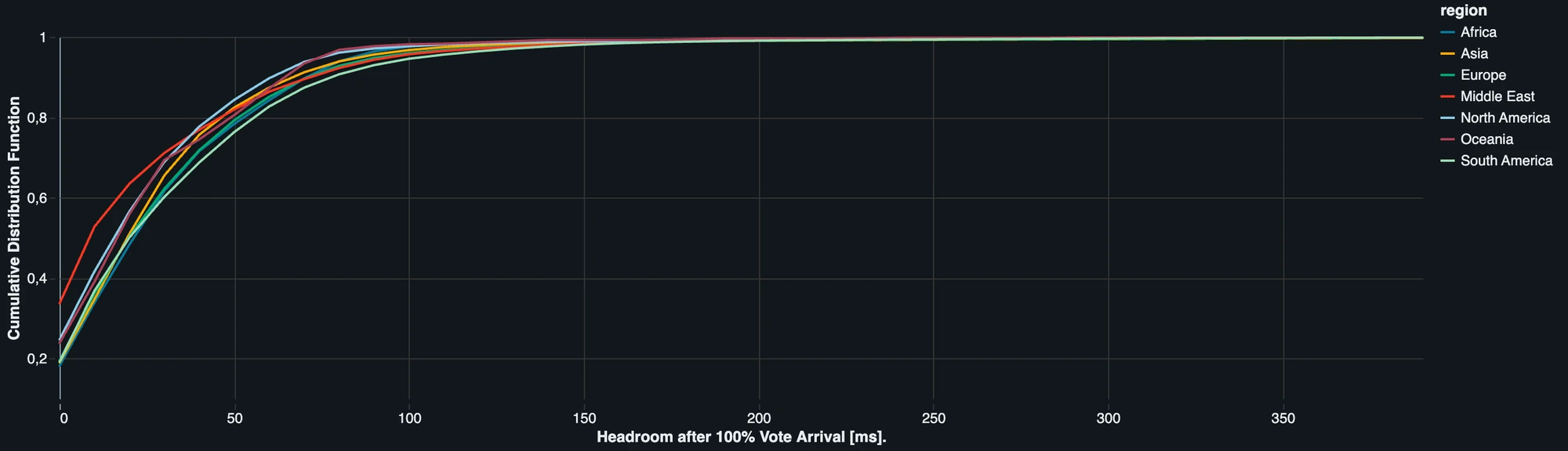
**Fig. 11:** **Remaining slot-time headroom after the final observed vote transaction, by region.** CDF of the difference between measured slot completion and the time at which 100% of the slot's observed vote transactions have arrived, grouped by region. The x-axis is remaining headroom in milliseconds; the y-axis is the cumulative fraction of observations with headroom at or below that value.

This makes attribution difficult. A late vote can reflect the validator's own voting policy, the client implementation, network propagation, or the leader's transaction-processing path. Current client heterogeneity means that the figure cannot identify which component is responsible.

That distinction is essential for TVC economics. If the relevant absolute delays remain unchanged while slot time is halved, some votes can move into later TVC latency buckets. But the present data cannot determine how much of the observed timing is fixed network latency and how much would adapt with the slot target.

A rough estimate of decreasing slot time on TVC has been given by Cavey here. From this analysis, it results that more than half of validators can expect about 1-2 bp reduction, while many other validators can expect up to 5 bp. A few validators in remote regions can expect 26-200 bps. It is worth noting that, this estimate is purely based on PoH tick data, removing knowledge of wall-clock time. This remains an upper bound if we consider that at the moment most validators are producing < 400ms slots.

Leader handoff as latency budget

Vote timing is only one part of the compressed latency budget. A second component appears at leader transitions.

Solana assigns four consecutive slots to a leader. The first slot of a new leader window - slot mod 4 = 0 - requires a handoff from the previous leader, whereas slots 1-3 are produced by the same leader.

Figure 12 isolates the additional duration associated with this transition. For each valid four-slot sequence, we define the time delta between the measured duration of the new leader's first slot and the mean value of the subsequent three. Positive values means the handoff slot was slower than that leader's within-window baseline.

Leader pairs are grouped by the Haversine distance between their reported geographic coordinates. The broad pattern is consistent with a distance-related handoff cost. Median difference rises from approximately 28 ms below 500 km to 35 ms at 500-1,000 km and 41 ms at 1,000-2,000 km. The 8,000+ km group reaches roughly 122 ms.

The relationship is not monotonic. The 2,000-4,000 km bin has a median penalty of approximately 101 ms, substantially above the neighboring 4,000-8,000 km bin at approximately 54 ms.

This anomaly is not explained by a small sample. The 2,000-4,000 km group contains 37,836 leader-window sequences, 483 current validators and 480 previous validators, with observer coverage comparable to the other bins.

Instead, its composition is unusual. Approximately 84% of the bin consists of US→US, US→CA, and CA→US transitions. Within US→US alone, the result is spread across thousands of directional validator pairs but remains materially concentrated among a subset of current leaders. Even more importantly, the same validator pair can exhibit very different handoff penalties when the direction is reversed, despite having exactly the same Haversine distance.

Figure 12 suggests a distance-dependent component to leader handoff latency, but it does not identify geographic distance as its cause. Haversine distance is only a proxy for network distance; routing, peering, data-center topology, client behavior, and leader-specific infrastructure remain unobserved.

This distinction becomes more important at 200 ms. A 100 ms handoff penalty consumes one quarter of a 400 ms target but one half of a 200 ms target. Even if average throughput remains unchanged, the tail of the handoff distribution can therefore become a materially larger fraction of the available block-production interval.

Appendix A - Slot-Level Model of Sandwich Profitability

This appendix extends the timing model to include market-local contention, residual slippage, attack costs, and imperfect ordering.

Transaction Contention

Let $\tau$ denote slot duration. Assume that transactions capable of moving the same market as the victim arrive according to a Poisson process with rate $\lambda$ . The expected number of relevant competing transactions during a slot is therefore

\mu = \lambda \tau.

The relevant arrival rate is market-local rather than network-wide transaction throughput.

Conditional on observing $N=n$ competing transactions, assume that the victim is exchangeable with them in execution order. If $K$ denotes the number of relevant transactions executed before the victim, then

K \mid N=n \sim \mathrm{Uniform}\{0,\dots,n\}.

After marginalizing over $N \sim \mathrm{Poisson}(\mu)$ , the marginal distribution of $K$ is

P(K=k) = \frac{1 - F_k(\mu)}{\mu},

where $F_k(\mu)$ is the Poisson CDF evaluated at $k$ .

Slot duration therefore affects pre-victim contention through $\mu=\lambda\tau$ : shorter slots reduce the expected number of relevant transactions that can precede the victim.

Remaining slippage and attack profitability

Let $s$ denote the victim's slippage tolerance and let $\gamma$ denote the average adverse price movement caused by one relevant transaction executed before the victim. After $K=k$ transactions, the remaining slippage headroom is

h_k = (s- k\gamma)_+.

Let $V$ denote the victim notional, let $\alpha$ denote the fraction of this headroom that can be converted into attacker revenue, and let $C$ denote the fixed cost of executing the sandwich. Conditional net profit is therefore

\pi_k = \left[\alpha V(s-k\gamma)-C\right]_+.

Define

c = \alpha Vs- C\ \qquad\text{and}\qquad\ b = \alpha V\gamma.

Then profit can be written more compactly as

\pi_k = (c-bk)_+.

A sandwich remains profitable only while

k \le m,\ \qquad\ m = \left\lfloor \frac{c}{b} \right\rfloor.

Timing and ordering

Let the victim arrive uniformly during the slot and let $d$ be the attacker's reaction latency. If a leader can hold the victim and execute it later in the same slot, the attacker only needs to submit before the slot closes. Temporal feasibility is therefore

p_{\mathrm{time}} = \left(1-\frac{d}{\tau}\right)_+.

Timely submission does not guarantee the desired front-run–victim–back-run ordering. Introduce therefore $q \in [0,1]$ , the conditional probability that the required ordering is obtained. This parameter absorbs scheduler behavior, fee and tip competition, bundle inclusion, and other ordering mechanisms not modeled explicitly.

Expected sandwich profit

Define the two partial Poisson sums

A_0(m,\mu)=\mu F_m(\mu)+(m+1)\left[1-F_{m+1}(\mu)\right]

and

A_1(m,\mu)=\frac{\mu^2}{2}F_{m-1}(\mu)+\frac{m(m+1)}{2}\left[1-F_{m+1}(\mu)\right].

Then expected net sandwich profit is

\Pi=q\left(1-\frac{d}{\tau}\right)_+\frac{cA_0(m,\mu)-bA_1(m,\mu)}{\mu},

provided that $c>0$ . If $c\le 0$ , then $\Pi=0$ .

For simulation, it is convenient to normalize by $\alpha V \gamma$ . Define

D = \frac{s}{\gamma},\ \qquad\ \phi = \frac{C}{\alpha V \gamma},\ \qquad\ \rho = \frac{d}{\tau}.

Under these definitions,

m = \lfloor D-\phi \rfloor\,,

and normalized expected profit becomes

\frac{\Pi}{\alpha V\gamma}=q(1-\rho)_+\frac{(D-\phi)A_0(m,\mu)-A_1(m,\mu)}{\mu}.

The corresponding probability of a profitable, timely, and correctly ordered attack is

P_{\mathrm{attack}}=q\left(1-\frac{d}{\tau}\right)_+\frac{A_0(m,\mu)}{\mu}.

Interpretation

Slot duration enters through two distinct mechanisms:

\mu = \lambda\tau\qquad\text{and}\qquad\rho = \frac{d}{\tau}.

Reducing $\tau$ lowers $\mu$ . Fewer relevant transactions are expected to execute before the victim, leaving more of its original slippage tolerance available when it is reached. Holding $s$ fixed, this tends to increase the amount available for extraction.

At the same time, reducing $\tau$ increases $\rho$ . The attacker has less time to observe the victim, construct its transactions, and submit them before the slot closes. This tends to reduce attack feasibility.

The two effects therefore work in opposite directions. The model does not imply that shorter slots mechanically reduce sandwich profitability.

A further effect can arise if users reduce slippage tolerance as contention falls. Since

E[K] = \frac{\lambda\tau}{2},

one simple behavioral closure is

D(\tau) = D_0 + \kappa \frac{\lambda\tau}{2},

where $D_0$ is the baseline slippage-to-impact ratio and $\kappa$ governs how strongly users adjust slippage to expected contention. Under this closure, shorter slots can additionally reduce the slippage exposed by the victim. This parameter, however, describes user behavior and must be calibrated rather than assumed.

Model boundary

The model is a sensitivity framework rather than an empirical estimate of realized sandwich MEV. It assumes Poisson market-local arrivals, exchangeable victim position, constant average price impact $\gamma$ , fixed reaction latency $d$ , and an exogenous ordering probability $q$ . The temporal condition also assumes that a victim can remain available for ordering until the end of the slot.

Consequently, the model isolates the channels through which slot duration can affect sandwich profitability, but it cannot determine the magnitude of the realized effect without calibrating market-local transaction intensity, slippage settings, price impact, attacker costs, reaction latency, and ordering behavior.